Prelim 2 Review and Simulation-Optimization


Lecture 20

December 3, 2025

Prelim 2 Review

Overall Statistics

  • Mean: 43.6/50 (87%)
  • Median: 45/50 (90%)
  • Standard Deviation: 6.2/50 (12%)

Alternatives to Mathematical Programming

Why Might We Want Alternatives?

Mathematical programming requires a particular geometry to ensure solutions or error guaranteed (e.g. linearity).

Many problems can be formulated in these frameworks, but not all…

What are some alternatives?

Generalized Search Algorithms

Function with Multiple Minima

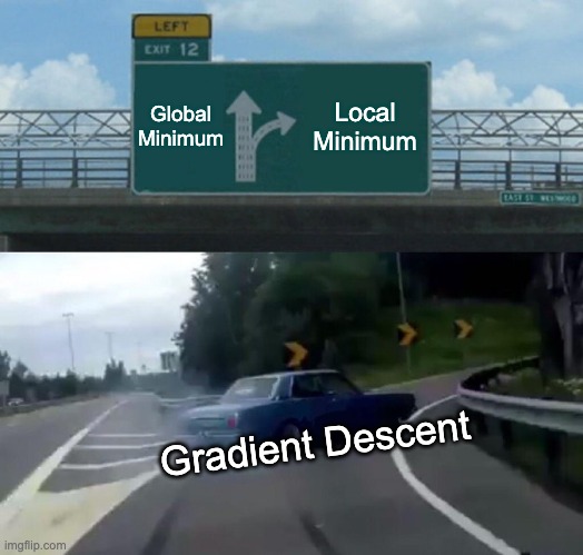
Most search algorithms look for critical points to find candidate optima. Then the “best” of the critical points is the global optimum.

Generalized Search Algorithms

Function with Multiple Minima

Two common approaches:

  • Gradient-based methods
  • Evolutionary algorithms

Gradient Descent

Find estimate of gradient near current point and step in positive/negative direction (depending on max/min).

\[x_{n+1} = x_n \pm \alpha_n \nabla f(x_n)\]

Gradient Descent: Challenges

  1. Need to tune stepsize for convergence; some use adaptive methods;
  2. May not have information about the gradient.

The second is more problematic: in some cases, methods like stochastic gradient approximation or automatic differentiation can be used.

Random Search with Constraints

Can also incorporate constraints into search.

Random Search in Julia

Two main packages:

Quick Example

Random.seed!(1)
# define function to optimize
function f(x)
    lnorm = LogNormal(0.25, 1) 
    y = rand(lnorm)
    return sum(x .- y)^2
end
fobj(x) = mean([f(x) for i in 1:1000])
bounds = [0.0 1000.0]'
# optimize
results = Metaheuristics.optimize(fobj, bounds, DE())
results.best_sol
(f = 3.7745e+00, x = [1.74764])

Metaheuristics.jl Algorithms

Metaheuristics.jl contains a number of algorithms, covering a variety of single-objective and multi-objective algorithms.

We won’t go into details here, and will just stick with DE() (differential evolution) in our examples.

Drawbacks of Search Algorithms

These methods work pretty well, but can:

  • require a lot of evaluations;
  • may get stuck at local optima;
  • may not converge if step sizes aren’t set correctly

waiting model evaluation meme

Generalized Search Algorithms

These methods work pretty well, but can:

  • require a lot of evaluations;
  • may get stuck at local optima;
  • may not converge if step sizes aren’t set correctly

waiting model evaluation meme

Generalized Search Algorithms

These methods work pretty well, but can:

  • require a lot of evaluations;
  • may get stuck at local optima;
  • may not converge if not tuned well.

waiting model evaluation meme

Simulation-Optimization

Simulation-Optimization

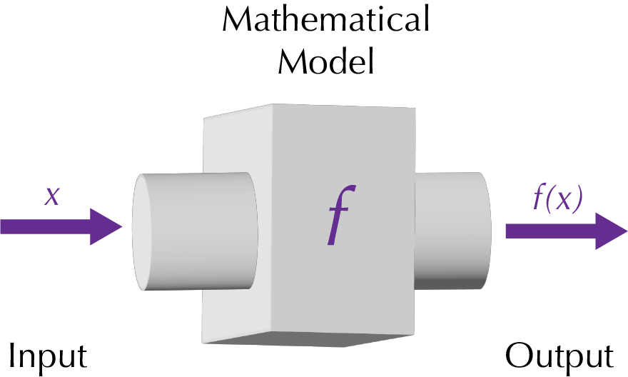
Simulation-Optimization involves the use of a simulation model to map decision variables and other inputs to system outputs.

Mathematical Model

Methods for Simulation-Optimization

What kinds of methods can use for simulation-optimization?

Mathematical Model

Simulation-Optimization: Methods

Challenge: Underlying structure of the simulation model \(f(x)\) is unknown and can be complex.

We can use a search algorithm to navigate the response surface of the model and find an “optimum”.

Mathematical Model

Why “Optimum” in Quotes?

We usually can’t guarantee that we can find an optimum (or even quantify an optimality gap) because:

  • Simulation-optimization is applied in very general settings;
  • May not have much a priori information about the response surface;
  • The response surface can be highly nonlinear.

Why “Optimum” in Quotes?

But:

The optimal solution of a model is not an optimal solution of a problem unless the model is a perfect representation of the problem, which it never is.

— Ackoff, R. L. (1979). “The Future of Operational Research is Past.” The Journal of the Operational Research Society, 30(2), 93–104. https://doi.org/10.1057/jors.1979.22

Simulation-Optimization and Heuristics

Simulation-optimization methods typically rely on heuristics to decide that a solution is good enough. These can include

  • number of evaluations/iterations; or
  • lack of improvement of solution with increased evaluations.

Lake Problem Revisited

Lake Model

\[\begin{align*} X_{t+1} &= X_t + a_t + y_t \\ &\quad + \frac{X_t^q}{1 + X_t^q} - bX_t,\\[0.5em] y_t &\sim \text{LogNormal}(\mu, \sigma^2) \end{align*}\]

Parameter Definition
\(X_t\) P concentration in lake
\(a_t\) point source P input
\(y_t\) non-point source P input
\(q\) P recycling rate
\(b\) rate at which P is lost

Lake Problem: Simulation-Optimization Setup

  • Time period: \(T=100\)
  • Non-point source P inflows: \(y_t \sim \text{LogNormal}(0.03, 0.25).\)
  • \(b = 2.5\) (P recycling rate), \(q=0.4\) (P outflow rate)
  • Constraint: \(\mathbb{P}[\text{Eutrophication}] \leq 0.1\)
  • Objective: Maximize average point source P releases \(\sum_t a_t / T\).

Lake Problem: Exogenous P Input Distribution

Lake Problem: Optimization Setup

  1. Set parameters and number of samples for exogenous inflows (we’ll use 1,000);
  2. Define model function and bounds (we’ll assume \(0 \leq a_t \leq 0.1\));
  3. Simulate objective and whether constraint is violated;
  4. Return objective and constraint status.
  5. Call optimizer (we’ll use DE() with a maximum of 10,000 function evaluations).

Lake Problem: Optimization Result

What do you observe?

Code
# find critical value


crit(x) = (x^q/(1+x^q)) - b*x
Xcrit = find_zero(crit, (0.1, 1.5))

function lake(a, y, q, b, T)
    X = zeros(T+1, size(y, 2))
    # calculate states
    for t = 1:T
        X[t+1, :] = X[t, :] .+ a[t] .+ y[t, :] .+ (X[t, :].^q./(1 .+ X[t, :].^q)) .- b.*X[t, :]
    end
    return X
end

function lake_opt(a, y, q, b, T, Xcrit)
    X = lake(a, y, q, b, T)
    # calculate exceedance of critical value
    Pexceed = sum(X[101, :] .> Xcrit) / size(X, 2)
    failconst = [Pexceed - 0.1]
    return mean(a), failconst, [0.0]
end

# set bounds
bounds = [0.0ones(T) 0.1ones(T)]'
# optimize
obj(a) = lake_opt(a, y, q, b, T, Xcrit)
options = Options(f_calls_limit=10_000)
results = Metaheuristics.optimize(obj, bounds, DE(options=options))

a = results.best_sol.x
pa = plot(a, tickfontsize=16, guidefontsize=16, ylabel="Point Source P Release", xlabel="Time", linewidth=3, legend=false, left_margin=5mm, bottom_margin=10mm)

End-Of-Time P Concentrations

Now we can simulate to learn about how the solution performs.

Code
X = lake(a, y, q, b, T)

histogram(X[101, :], xlabel="End P Concentration", ylabel="Count",
    guidefontsize=16, tickfontsize=16, 
    legendfontsize=16, label=:false, bottom_margin=5mm, left_margin=5mm)
vline!([Xcrit], color=:red, linestyle=:dot, 
    label="Critical Value")
    plot!(size=(1000, 450))

Lake P Concentration Trajectories

Code
pconc = plot(X, alpha=0.2,  linewidth=3,
    guidefontsize=16, tickfontsize=16, 
    legendfontsize=16, label=:false,
    legend=:topleft, bottom_margin=10mm, left_margin=5mm, grid=false)
hline!([Xcrit], color=:red, linestyle=:dot, 
    label="Critical Value")
plot!(size=(600, 600))
ylabel!("Lake P Concentration")
xlabel!("Time")
  • Trajectories start jumping over the critical threshold later in the horizon.
  • This finite horizon problem is very common for optimization problems with reliability constraints over fixed temporal windows.

Heuristic Algorithms Involve Lots of Choices!

Many choices were made in this optimization problem:

  • Number of samples from the inflow distribution;
  • Number of function evaluations;
  • Strength of reliability constraint.

All of these affect the tradeoff between solution quality and computational expense.

Dimension Reduction via Decision Rules

Optimization converges faster with fewer variables.

Instead of optimizing the entire sequence of decisions, formulate those decisions as a decision rule \(a_t = f(X_{t}).\)

Example: Quinn et al. (2017) uses \[a_t = \min\left(\max\left(\sum_j w_j \left| \frac{X_t - c_j}{r_j}\right|^3, 0.01\right), 0.1\right).\]

Key Takeaways

General Takeaways

  • Many challenges to using mathematical programming for general systems analysis.
  • Can use simulation-optimization approaches.
  • Tradeoff between lack of analytic solution and broader flexibility
  • But be careful of computational expense and convergence!

Challenges to Simulation-Optimization in General

  • Monte Carlo Error: If constraints or objective is probabilistic, how many Monte Carlo runs are needed to ensure difference in function values is “real” and not stochastic noise.
  • Computational: Can be expensive depending on the simulation model.
  • Local vs. Global Optima: Depending on type of search algorithm, may not be able to guarantee more than a local optimum.
  • Transparency: LP models are written down relatively clearly. Simulation models may have many important but hidden assumptions.

Class Wrap-Up

Content

  • What is a system? Why are they challenging to understand?
  • Simulation to understand system dynamics.
  • Optimization to make decisions about managing systems.
  • Sensitivity Analysis: What matters?

Themes

  • Systems can be complex: often require models to make sense of how they behave and respond to different inputs.
  • Models necessarily are approximations to reality: be mindful of when these are appropriate and when they are too strong.
  • Modeled results from a sound model are good starting points for further interrogation. Please do not treat them as the end point!

Upcoming Schedule

Upcoming Schedule

No Class Monday:

HW5: Due tomorrow (12/4)

Project Deadlines

  • Submit presentation videos to Canvas by midnight Monday (cannot be late or you will not be assigned peer reviews).
  • Peer reviews will be assigned Tuesday, due by Thursday evening.
  • Final reports due end of finals week (12/20).
  • Team and self Evaluations due end of finals week (12/20).
Quinn, J. D., Reed, P. M., & Keller, K. (2017). Direct policy search for robust multi-objective management of deeply uncertain socio-ecological tipping points. Environmental Modelling & Software, 92, 125–141. https://doi.org/10.1016/j.envsoft.2017.02.017