Sensitivity Analysis
Lecture 19
November 24, 2025
How High Will CO2 Emissions Be In 2100?

Text: VSRIKRISH to 22333
Translating the Word Salad
- Known Knowns: Certainty
- Known Unknowns: “Shallow” Uncertainty
- Unknown Unknowns: “Deep” Uncertainty or ambiguity

Prioritizing Factors Of Interest
- How do we know which factors are most relevant to a particular analysis?
- What modeling assumptions were most responsible for output uncertainty?

Source: Saltelli et al (2019)
Why Perform Sensitivity Analysis?
Source: Reed et al (2022)
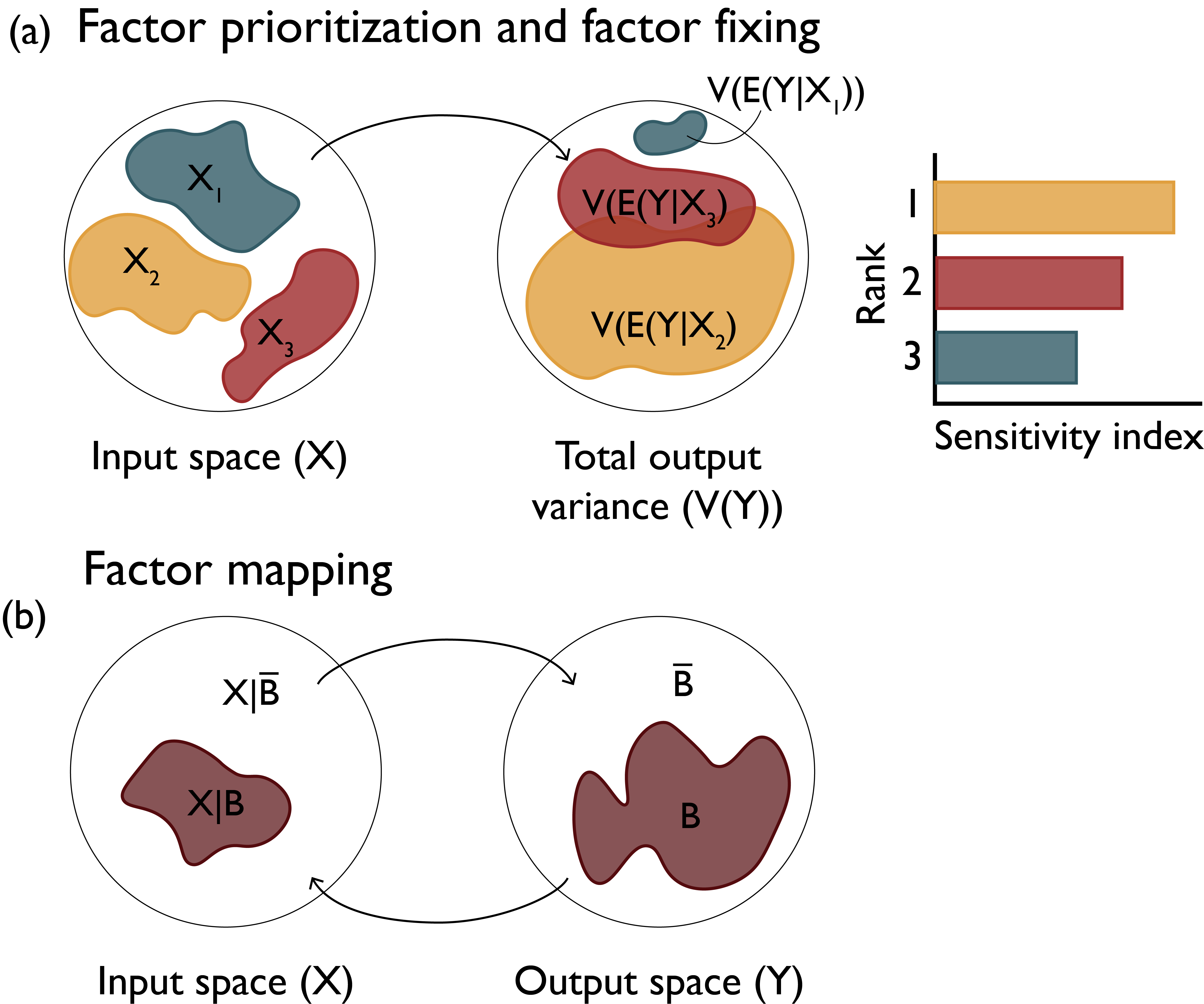
Factor Prioritization
Which factors have the greatest impact on output variability?
Source: Reed et al (2022)
Factor Fixing
Which factors have negligible impact and can be fixed in subsequent analyses?
Source: Reed et al (2022)
Factor Mapping
Which values of factors lead to model outputs in a certain output range?
Source: Reed et al (2022)
Local SA
Local sensitivities: Pointwise perturbations from some baseline point.
Challenge: Which point to use?
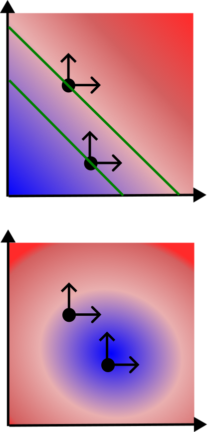
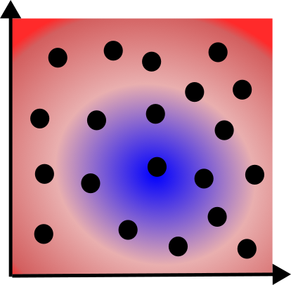
Global SA
Global sensitivities: Sample throughout the space.
Challenge: How to measure global sensitivity to a particular output?
Advantage: Can estimate interactions between parameters
Parameter Interactions
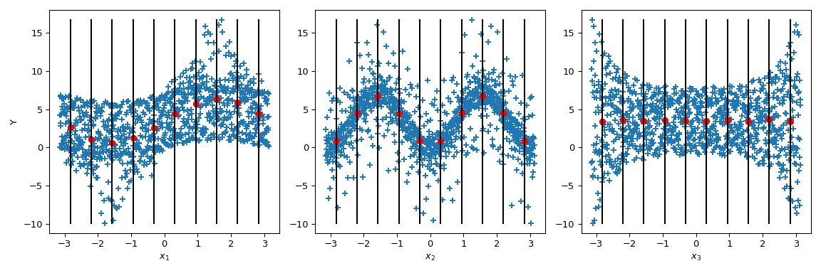
Source: SciPy Documentation
Example: Cumulative CO2 Emissions
Think about the joint population-economic-emissions system:
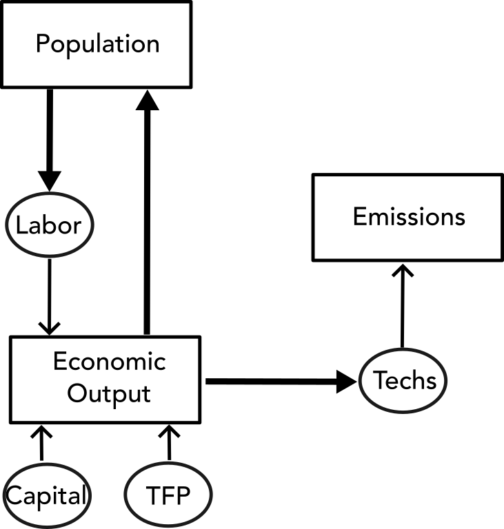
Example: Cumulative CO2 Emissions
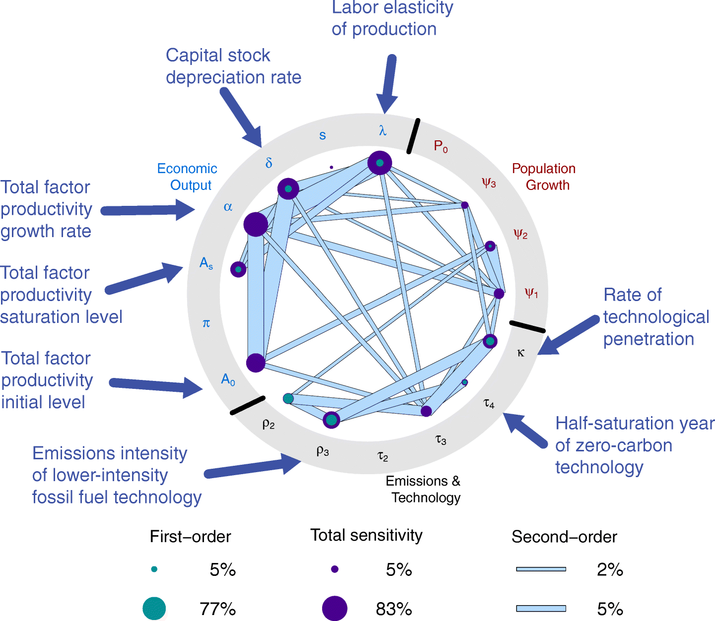
Source: Srikrishnan et al (2022)