System Dynamics: Equilibria and Bifurcations

---

Lecture 05

September 10, 2024

Overview

• Review of Last Class
• Equilibria
• Shallow Lake Model
• Equilibria and Bifurcations
• Key Takeaways
• Upcoming Schedule
• References

Review of Last Class

Feedbacks

Feedbacks are “loops” in a system diagram.

Feedbacks can be:

• Amplifying (sometimes called “positive”)
• Dampening (sometimes called “negative”)

Ice-Albedo Feedback Loop

Amplifying Feedbacks

Shocks will amplify as they are propagated:

Amplifying Feedback Example

Dampening Feedbacks

Shocks are attenuated (dampened) as they propagate:

Dampening Feedback Example

Questions?

Text: VSRIKRISH to 22333

URL: https://pollev.com/vsrikrish

See Results

Equilibria

Fixed Points (Equilibria)

System dynamics are often understood relative to their equilibria (or fixed points).

• If \(X_{t+1} = F(X_t)\), equilibria occur where \(F(X_t) = X_t\).
• If \(\frac{dx}{dt} = f(x)\), equilibria occur where \(f(x) = 0\).

In other words, a system at an equilibrium will stay at an equilibrium.

Example: Predator-Prey Dynamics

lh_obs = DataFrame(CSV.File("data/lynx_hare/Lynx_Hare.txt", header=[:Year, :Hare, :Lynx]))[:, 1:3]
plot(lh_obs[!, :Year], lh_obs[!, :Lynx], xlabel="Year", ylabel="Pelts (thousands)", markersize=5, markershape=:circle, markercolor=:red, color=:red, linewidth=3, label="Lynx")
plot!(lh_obs[!, :Year], lh_obs[!, :Hare], markersize=5, markershape=:circle, markercolor=:blue, color=:blue, linewidth=3, label="Hare")
plot!(size=(1100, 500))

Figure 1: Lynx and Hare pelt dataset

Predator-Prey Dynamics (Lotka-Volterra)

\[ \begin{align*} \frac{dH}{dt} &= H_t \underbrace{b_H}_{\substack{\text{birth} \\ \text{rate}}} - H_t (\underbrace{L_t m_H}_{\substack{\text{impact of} \\ \text{lynxes}}}) \\ \frac{dL}{dt} &= L_t (H_t b_L)_{\substack{\text{impact of} \\ \text{hares}}}) - \underbrace{L_t m_L}_{\substack{\text{mortality} \\ \text{rate}}}) \end{align*} \]

Lotka-Volterra Fixed Points

function lotka_volterra!(du, u, p, t)
  # Unpack the values so that they have clearer meaning
  prey, pred  = u
  birth_prey, mort_prey, birth_pred, mort_pred = p

  # Define the ODE
  du[1] = (birth_prey - mort_prey * pred) * prey
  du[2] = (birth_pred * prey - mort_pred) * pred
end

# define model parameters and initial conditions
θ = [1.1, 0.5, 0.1, 0.2]
u₀ = [1, 1]
tspan = 40
prob = ODEProblem(lotka_volterra!, u₀, (0.0, tspan), θ)


# plot phase space
p = plot(xlims=(0, 10), ylims=(0, 6),
    xlabel = "Prey Population (1,000)", ylabel = "Predator Population (1,000)", leg = false)

function phase_plot(prob, u0, θ, p, tspan = 40)
    _prob = ODEProblem(prob.f, u0, tspan, θ)
    sol = solve(_prob, Vern9()) # Use Vern9 solver for higher accuracy
    plot!(p, sol, idxs = (1, 2))
end

for x in 0:0.5:2.5
    for y in 0:0.5:2.5
        phase_plot(prob, [y, x], θ, p)
    end
end

scatter!(p, [0, 2], [0, 2.2], color=:black)
plot!(size=(650, 550))

Figure 2: Phase Diagram of the Lotka-Volterra Equations

This simple model has two fixed points:

1. \(L_t = 0, H_t = 0\)
2. \(L_t = b_H / m_H, H_t = m_L / b_L\)

Stability

Equilibria can be stable or unstable.

Initial Conditions Diagram

Shallow Lake Model

Shallow Lake Model

• Model introduced by Carpenter et al. (1999).
• This lecture builds off Quinn et al. (2017).
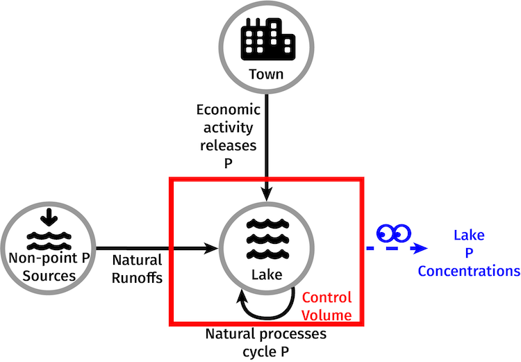
• Tradeoff between economic benefits and the health of the lake.

Lake Eutrophication Example

Shallow Lake Model: Variables

Variable	Meaning	Units
\(X_t\)	P level in lake at time \(t\)	dimensionless
\(a_t\)	Controllable (point-source) P release	dimensionless
\(y_t\)	Random (non-point-source) P runoff	dimensionless

Shallow Lake Model: Runoff

Random runoffs \(y_t\) are sampled from a LogNormal distribution.

# this uses StatsPlots.jl's recipe for plotting distributions directly; otherwise use something like plot(-5:0.01:5, pdf.(LogNormal(0.25, 1), -5:0.1:5))
plot(LogNormal(0.25, 1), linewidth=3, label="LogNormal(0.25, 1)")
plot!(LogNormal(0.5, 1), linewidth=3, label="LogNormal(0.5, 2)")
plot!(LogNormal(0.25, 2), linewidth=3, label="LogNormal(0.25, 2)")
plot!(size=(1000, 400), grid=:false, left_margin=10mm, right_margin=10mm, bottom_margin=10mm)
xlims!((0, 6))
ylabel!("Density")
xlabel!(L"y_t")

Figure 3: Lognormal Distributions

Shallow Lake Model: P Dynamics

• Lake loses P at a linear rate, \(bX_t\).
• Nutrient cycling reintroduces P from sediment: \[\frac{X_t^q}{1 + X_t^q}.\]

Shallow Lake Model

So the P level (state) \(X_{t+1}\) is given by: \[\begin{gather*} X_{t+1} = X_t + a_t + y_t + \frac{X_t^q}{1 + X_t^q} - bX_t, \\[0.5em] y_t \underset{\underset{\Large\text{\color{red}sample}}{\color{red}\uparrow}}{\sim} \text{LogNormal}(\mu, \sigma^2). \end{gather*} \]

Equilibria and Bifurcations

Lake Dynamics (Without Inflows)

• \(a_t = y_t = 0\),
• \(q=2.5\)
• \(b=0.4\)

# define functions for lake recycling and outflows
lake_P_cycling(x, q) = x.^q ./ (1 .+ x.^q);
lake_P_out(x, b) = b .* x;

T = 30
X_vals = collect(0.0:0.1:2.5)
function simulate_lake_P(X_ic, T, b, q, a, y)
    X = zeros(T)
    X[1] = X_ic
    for t = 2:T
        X[t] = X[t-1] .+ a[t] .+ y[t].+ lake_P_cycling(X[t-1], q) .- lake_P_out(X[t-1], b)
    end
    return X
end
X = map(x -> simulate_lake_P(x, T, 0.4, 2.5, zeros(T), zeros(T)), X_vals)
p_noinflow = plot(X, label=false, ylabel=L"X_t", xlabel="Time", size=(600, 500))

Figure 4: Dynamics of lake model with different initial conditions

Lake Dynamics (Without Inflows)

• \(a_t = y_t = 0\),
• \(q=2.5\)
• \(b=0.4\)

# define range of lake states X
x = 0:0.05:2.5;

# plot recycling and outflows for selected values of b and q
p1 = plot(x, lake_P_cycling(x, 2.5), color=:black, linewidth=5,legend=:topleft, label="P Recycling", ylabel="P Flux", xlabel=L"$X_t$", palette=:tol_muted, framestyle=:zerolines, grid=:false)
plot!(x, lake_P_out(x, 0.4), linewidth=3, linestyle=:dash, label="b=0.4", color=:blue)
quiver!([1], [0.35], quiver=([1], [0.4]), color=:red, linewidth=2)
quiver!([0.4], [0.13], quiver=([-0.125], [-0.05]), color=:red, linewidth=2)
quiver!([2.5], [0.97], quiver=([-0.125], [-0.05]), color=:red, linewidth=2)
plot!(ylims=(-0.02, 1.1))
plot!(size=(600, 500))

Figure 5: Lake eutrophication dynamics based on the shallow lake modelwithout additional inputs. The black line is the P recycling level (for $q=2.5), which adds P back into the lake, and the dashed lines correspond to differerent rates of P outflow (based on the linear parameter \(b\)). The lake P level is in equilibrium when the recycling rate equals the outflows. When the outflow is greater than the recycling flux, the lake’s P level decreases, and when the recycling flux is greater than the outflow, the P level naturally increases. The red lines show the direction of this net flux.

Where Are the Equilibria?

Equilibria: Fixed points of the dynamics (no state change).

Equilibria occur where \[\Delta X = X_{t+1} - X_t = 0,\] so the outflows and sediment recycling are in balance.

eq1 = [0.0, 0.67, 2.2]
scatter!(p1, eq1, (y -> lake_P_cycling(y, 2.5)).(eq1), label="Equilibria", markersize=10, markercolor=:blue)

Figure 6: Lake eutrophication dynamics based on the shallow lake modelwithout additional inputs. The black line is the P recycling level (for \(q=2.5\)), which adds P back into the lake, and the dashed lines correspond to differerent rates of P outflow (based on the linear parameter \(b\)). The lake P level is in equilibrium when the recycling rate equals the outflows. When the outflow is greater than the recycling flux, the lake’s P level decreases, and when the recycling flux is greater than the outflow, the P level naturally increases. The red lines show the direction of this net flux.

Stability of Equilibria

Consider a discrete system model \(X_{t+1} = F(X_t)\) (continuous: \(\frac{dx}{dt} = f(x)\)).

• An equilibrium \(X^*\) is stable if nearby points are attracted to it (small perturbations “recover”): \(|F'(X^*)| < 1\) or \(f'(X^*) < 0\)
• \(X^*\) is unstable if nearby points are repelled by it: \(|F'(X^*)| > 1\) or \(f'(X^*) > 0\)

Stability and Resilience

Can think of stable equilibria as suggesting “resilience”: small disruptions to the system state will fade away with time and the system will stabilize.

Unstable equilibria: small shocks amplify and the system will deviate from its “typical” state.

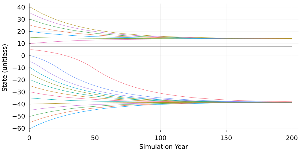
Implications of Unstable Equilibria

plot!(p_noinflow, title="Lake P Without Inflows", titlefontsize=20)

Figure 7: Dynamics of Lake Model With No Inflows

a = zeros(T)
y = rand(LogNormal(log(0.08), 0.01), T)
X = map(x -> simulate_lake_P(x, T, 0.4, 2.5, a, y), X_vals) 
plot(X, label=false, ylabel=L"$X_t$", xlabel="Time", title="Lake P With Inflows", size=(600, 500))

Figure 8: Dynamics of Lake Model With No Inflows

How do Equilibria Change?

How do the equilibria change as system parameters vary?

eq_45 = [0.8, 1.8]
eq_5 = [1.0, 1.4]
plot!(p1, x, lake_P_out(x, 0.45), linewidth=3, linestyle=:dash, label="b=0.45", color=:orange)
plot!(p1, x, lake_P_out(x, 0.5), linewidth=3, linestyle=:dash, label="b=0.5", color=:purple)
plot!(p1, x, lake_P_out(x, 0.6), linewidth=3, linestyle=:dash, label="b=0.6", color=:green)
scatter!(p1, eq_45, (y -> lake_P_cycling(y, 2.5)).(eq_45), label=false, markersize=10, markercolor=:orange)
scatter!(p1, eq_5, (y -> lake_P_cycling(y, 2.5)).(eq_5), label=false, markersize=10, markercolor=:purple)

Figure 9: Lake eutrophication dynamics based on the shallow lake modelwithout additional inputs. The black line is the P recycling level (for \(q=2.5\)), which adds P back into the lake, and the dashed lines correspond to differerent rates of P outflow (based on the linear parameter \(b\)). The lake P level is in equilibrium when the recycling rate equals the outflows. When the outflow is greater than the recycling flux, the lake’s P level decreases, and when the recycling flux is greater than the outflow, the P level naturally increases. The red lines show the direction of this net flux.

Equilibria vs. \(b\) Value

function plot_P_flux(b_vals)
    p = plot(; xlabel="b", ylabel="X", legend=:outerright, size=(1200, 500), leftmargin=10mm)

    flux_func(x, b) = lake_P_cycling(x, 2.5) - lake_P_out(x, b)
    X_un = []
    X_st = []
    for b in b_vals
        # try to find the unstable (oligotrophic) equilibrium
        try
            x_eq = Roots.find_zero(x -> flux_func(x, b), 0.5)
            push!(X_un, (b, x_eq))
        catch err
            if isa(err, DomainError)
            end
        end
        # try to find the stable (eutrophic) equilibrium
        try
            x_eq = Roots.find_zero(x -> flux_func(x, b), 2.0)
            push!(X_st, (b, x_eq))
        catch err
            if isa(err, DomainError)
            end
        end
    end
    plot!(p, first.(X_un), last.(X_un), label="Unstable Equilibrium", linewidth=3, color=:red, linestyle=:dash)
    plot!(p, first.(X_st), last.(X_st), label="Stable (Eutrophic) Equilibrium", linewidth=3, color=:red)
    plot!(p, b_vals, repeat([0.0], length(b_vals)), label="Stable (Oligotrophic) Equilibrium", linewidth=3, color=:blue)

    quiver!(p, [0.01], [0.15], quiver=([0.0], [5.85]), color=:black)
    quiver!(p, [0.05], [0.2], quiver=([0.0], [5.8]), color=:black)
    quiver!(p, [0.1], [0.4], quiver=([0.0], [5.6]), color=:black)
    quiver!(p, [0.15], [0.5], quiver=([0.0], [5.5]), color=:black)
    quiver!(p, [0.2], [0.5], quiver=([0.0], [4.0]), color=:black)
    quiver!(p, [0.25], [0.6], quiver=([0.0], [3.0]), color=:black)
    quiver!(p, [0.3], [0.6], quiver=([0.0], [2.4]), color=:black)
    quiver!(p, [0.35], [0.7], quiver=([0.0], [1.7]), color=:black)
    quiver!(p, [0.4], [0.8], quiver=([0.0], [1.3]), color=:black)
    quiver!(p, [0.45], [0.9], quiver=([0.0], [0.75]), color=:black)
    quiver!(p, [0.5], [1.1], quiver=([0.0], [0.25]), color=:black)

    quiver!(p, [0.1], [0.15], quiver=([0.0], [-0.15]), color=:black)
    quiver!(p, [0.15], [0.2], quiver=([0.0], [-0.15]), color=:black)
    quiver!(p, [0.2], [0.25], quiver=([0.0], [-0.2]), color=:black)
    quiver!(p, [0.25], [0.35], quiver=([0.0], [-0.3]), color=:black)
    quiver!(p, [0.3], [0.4], quiver=([0.0], [-0.35]), color=:black)
    quiver!(p, [0.35], [0.45], quiver=([0.0], [-0.4]), color=:black)
    quiver!(p, [0.4], [0.55], quiver=([0.0], [-0.45]), color=:black)
    quiver!(p, [0.45], [0.7], quiver=([0.0], [-0.6]), color=:black)
    quiver!(p, [0.5], [0.9], quiver=([0.0], [-0.8]), color=:black)

    quiver!(p, [0.2], [6.0], quiver=([0.0], [-0.9]), color=:black)
    quiver!(p, [0.25], [6.0], quiver=([0.0], [-2.0]), color=:black)
    quiver!(p, [0.3], [6.0], quiver=([0.0], [-2.7]), color=:black)
    quiver!(p, [0.35], [6.0], quiver=([0.0], [-3.2]), color=:black)
    quiver!(p, [0.4], [6.0], quiver=([0.0], [-3.8]), color=:black)
    quiver!(p, [0.45], [6.0], quiver=([0.0], [-4.0]), color=:black)
    quiver!(p, [0.5], [6.0], quiver=([0.0], [-4.5]), color=:black)
    quiver!(p, [0.55], [6.0], quiver=([0.0], [-5.9]), color=:black)
    quiver!(p, [0.6], [6.0], quiver=([0.0], [-5.9]), color=:black)

    return p
end
b_vals = 0.01:0.01:0.6

p = plot_P_flux(b_vals)
display(p)

Figure 10: Bifurcation diagram for the lake problem with no inputs.

Implications of Bifurcations

Bifurcations have the following implications:

• Uncertainty about system dynamics can dramatically change equilibria locations and behavior;
• “Shocks” (in this case, sedimentation/recycling disturbances or massive non-point source inflows) can irreversibly alter system outcomes.

Key Takeaways

Key Takeaways (Equilibria)

• System equilibria states can be stable or unstable.
• Unstable equilbria can be responsible for thresholds/tipping points.
• Bifurcations: Changes to number/qualitative behavior of equilibria as system properties vary.

Upcoming Schedule

Next Classes

Next Week: Simulation Models

Assessments

Homework 1: Due 9/11 at 9pm

References

References

Carpenter, S. R., Ludwig, D., & Brock, W. A. (1999). Management of eutrophication for lakes subject to potentially irreversible change. Ecol. Appl., 9(3), 751–771. https://doi.org/10.2307/2641327

Quinn, J. D., Reed, P. M., & Keller, K. (2017). Direct policy search for robust multi-objective management of deeply uncertain socio-ecological tipping points. Environmental Modelling & Software, 92, 125–141. https://doi.org/10.1016/j.envsoft.2017.02.017